Dynamic Effects with base_period = "universal"

This notebook shows how to estimate dynamic (event-study) treatment effects with the csdid package using the base_period = "universal" option of ATTgt.fit().

The base_period argument controls which pre-treatment period is used as the reference for each \(ATT(g,t)\):

• base_period = "varying" (default) — the base period changes with \(t\). For pre-treatment periods, the base is \(t-1\) (so pre-treatment \(ATT(g,t)\) resemble a placebo test in differences). For post-treatment periods, the base is the last period before \(g\) becomes treated.

• base_period = "universal" — the base period is fixed to the last pre-treatment period for every group (with anticipation accounted for). The \(ATT\) at the base period itself is normalized to zero. This matches the standard event-study normalization that fixes the level at \(e = -1\).

Both options give the same \(ATT(g,t)\) for post-treatment periods. They differ only in how pre-treatment \(ATT(g,t)\) are reported, which in turn changes the look of the event-study plot.

# pip install git+https://github.com/d2cml-ai/csdid/
# pip install git+https://github.com/d2cml-ai/DRDID
from csdid.att_gt import ATTgt
import pandas as pd
import warnings
warnings.filterwarnings('ignore')

Data

We use the same mpdta dataset (county-level teen employment, 2003-2007) used elsewhere in this site.

mpdta = pd.read_csv("https://raw.githubusercontent.com/d2cml-ai/csdid/main/data/mpdta.csv")
mpdta.head()

	year	countyreal	lpop	lemp	first.treat	treat
0	2003	8001	5.896761	8.461469	2007	1
1	2004	8001	5.896761	8.336870	2007	1
2	2005	8001	5.896761	8.340217	2007	1
3	2006	8001	5.896761	8.378161	2007	1
4	2007	8001	5.896761	8.487352	2007	1

Varying base period (default)

First, the default. base_period does not need to be specified.

mw_varying = ATTgt(
    yname="lemp",
    gname="first.treat",
    idname="countyreal",
    tname="year",
    xformla="lemp~1",
    data=mpdta,
).fit(est_method="dr", base_period="varying")

mw_varying.summ_attgt().summary2

	Group	Time	ATT(g, t)	Post	Std. Error	[95% Pointwise	Conf. Band]
0	2004	2004	-0.0105	1	0.0232	-0.0727	0.0517
1	2004	2005	-0.0704	1	0.0321	-0.1565	0.0157
2	2004	2006	-0.1373	1	0.0379	-0.2391	-0.0355	*
3	2004	2007	-0.1008	1	0.0357	-0.1967	-0.0049	*
4	2006	2004	0.0065	0	0.0245	-0.0594	0.0724
5	2006	2005	-0.0028	0	0.0193	-0.0545	0.0490
6	2006	2006	-0.0046	1	0.0172	-0.0507	0.0415
7	2006	2007	-0.0412	1	0.0196	-0.0938	0.0113
8	2007	2004	0.0305	0	0.0153	-0.0105	0.0716
9	2007	2005	-0.0027	0	0.0164	-0.0467	0.0412
10	2007	2006	-0.0311	0	0.0182	-0.0799	0.0177
11	2007	2007	-0.0261	1	0.0173	-0.0726	0.0205

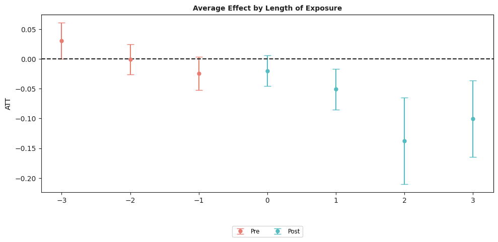
mw_varying.aggte(typec="dynamic")
mw_varying.plot_aggte();

Overall summary of ATT's based on event-study/dynamic aggregation:
    ATT Std. Error  [95.0%  Conf. Int.]
-0.0772     0.0221 -0.1205       -0.034 *


Dynamic Effects:
   Event time  Estimate  Std. Error  [95.0% Simult.   Conf. Band
0          -3    0.0305      0.0155           0.0002      0.0608  *
1          -2   -0.0006      0.0130          -0.0261      0.0250
2          -1   -0.0245      0.0142          -0.0522      0.0033
3           0   -0.0199      0.0132          -0.0458      0.0060
4           1   -0.0510      0.0173          -0.0848     -0.0171  *
5           2   -0.1373      0.0371          -0.2100     -0.0646  *
6           3   -0.1008      0.0327          -0.1650     -0.0366  *
---
Signif. codes: `*' confidence band does not cover 0
Control Group:  Never Treated ,
Anticipation Periods:  0
Estimation Method:  Doubly Robust

Universal base period

Now set base_period = "universal" in the call to fit. Everything else stays the same.

mw_universal = ATTgt(
    yname="lemp",
    gname="first.treat",
    idname="countyreal",
    tname="year",
    xformla="lemp~1",
    data=mpdta,
).fit(est_method="dr", base_period="universal")

mw_universal.summ_attgt().summary2

No units in group 2004 in time period 1, e2
No available control units for group 2004 in time period 1, e4
No units in group 2006 in time period 3, e2
No available control units for group 2006 in time period 3, e4
No units in group 2007 in time period 4, e2
No available control units for group 2007 in time period 4, e4

	Group	Time	ATT(g, t)	Post	Std. Error	[95% Pointwise	Conf. Band]
0	2004	2003	NaN	0	NaN	NaN	NaN
1	2004	2004	-0.0105	1	0.0248	-0.0771	0.0561
2	2004	2005	-0.0704	1	0.0334	-0.1599	0.0191
3	2004	2006	-0.1373	1	0.0385	-0.2406	-0.0339	*
4	2004	2007	-0.1008	1	0.0326	-0.1882	-0.0135	*
5	2006	2003	-0.0038	0	0.0320	-0.0895	0.0820
6	2006	2004	0.0028	0	0.0193	-0.0490	0.0545
7	2006	2005	NaN	0	NaN	NaN	NaN
8	2006	2006	-0.0046	1	0.0189	-0.0552	0.0460
9	2006	2007	-0.0412	1	0.0201	-0.0952	0.0127
10	2007	2003	0.0033	0	0.0265	-0.0678	0.0744
11	2007	2004	0.0338	0	0.0217	-0.0243	0.0919
12	2007	2005	0.0311	0	0.0182	-0.0176	0.0798
13	2007	2006	NaN	0	NaN	NaN	NaN
14	2007	2007	-0.0261	1	0.0166	-0.0706	0.0184

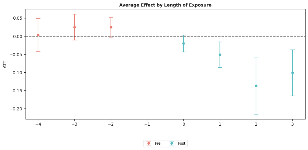
mw_universal.aggte(typec="dynamic")
mw_universal.plot_aggte();

Overall summary of ATT's based on event-study/dynamic aggregation:
    ATT Std. Error  [95.0%  Conf. Int.]
-0.0772     0.0209 -0.1182      -0.0363 *


Dynamic Effects:
   Event time  Estimate  Std. Error  [95.0% Simult.   Conf. Band
0          -4    0.0033      0.0233          -0.0424      0.0490
1          -3    0.0250      0.0183          -0.0108      0.0608
2          -2    0.0245      0.0139          -0.0028      0.0517
3           0   -0.0199      0.0119          -0.0433      0.0035
4           1   -0.0510      0.0182          -0.0865     -0.0154  *
5           2   -0.1373      0.0397          -0.2150     -0.0595  *
6           3   -0.1008      0.0326          -0.1646     -0.0370  *
---
Signif. codes: `*' confidence band does not cover 0
Control Group:  Never Treated ,
Anticipation Periods:  0
Estimation Method:  Doubly Robust