7. Linear Penalized Regs#
7.1. Data Generating Process: Approximately Sparse#
install.packages("librarian", quiet = T)
librarian::shelf(glmnet, broom, tidyverse, hdm, quiet = T)
set.seed(1)

n = 100;
p = 400;

Z= runif(n)-1/2;
W = matrix(runif(n*p)-1/2, n, p);


beta = 1/seq(1:p)^2;   # approximately sparse beta
#beta = rnorm(p)*.2    # dense beta
gX = exp(4*Z)+ W%*%beta;  # leading term nonlinear
X = cbind(Z, Z^2, Z^3, W );  # polynomials in Zs will be approximating exp(4*Z)


Y = gX + rnorm(n);    #generate Y


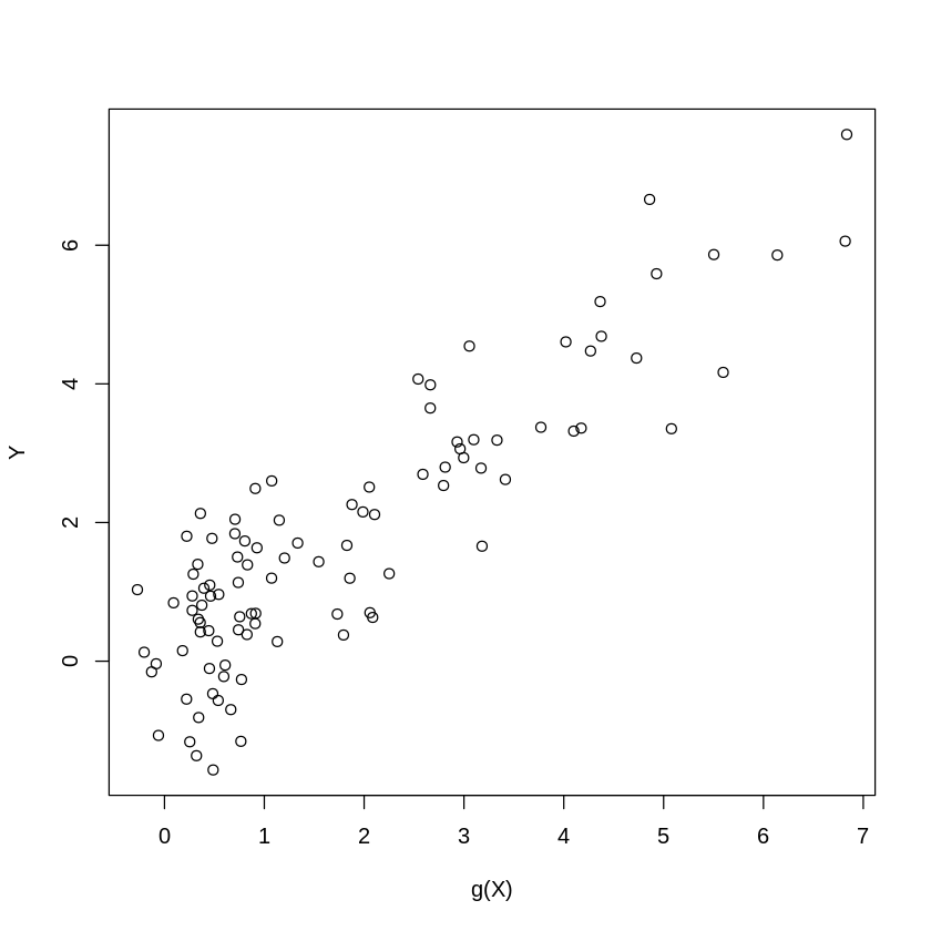
plot(gX,Y, xlab="g(X)", ylab="Y")    #plot V vs g(X)

print(c("theoretical R2:", var(gX)/var(Y)))
Warning message in system("timedatectl", intern = TRUE):
“running command 'timedatectl' had status 1”
[1] "theoretical R2:" "0.826881788964026"
| 0.8268818 |

We use package Glmnet to carry out predictions using cross-validated lasso, ridge, and elastic net
# library(glmnet)
fit.lasso.cv   <- cv.glmnet(X, Y, family="gaussian", alpha=1)  # family gaussian means that we'll be using square loss
fit.ridge   <- cv.glmnet(X, Y, family="gaussian", alpha=0)     # family gaussian means that we'll be using square loss
fit.elnet   <- cv.glmnet(X, Y, family="gaussian", alpha=.5)    # family gaussian means that we'll be using square loss

yhat.lasso.cv    <- predict(fit.lasso.cv, newx = X)            # predictions
yhat.ridge   <- predict(fit.ridge, newx = X)
yhat.elnet   <- predict(fit.elnet, newx = X)

MSE.lasso.cv <- summary(lm((gX-yhat.lasso.cv)^2~1))$coef[1:2]  # report MSE and standard error for MSE for approximating g(X)
MSE.ridge <- summary(lm((gX-yhat.ridge)^2~1))$coef[1:2]        # report MSE and standard error for MSE for approximating g(X)
MSE.elnet <- summary(lm((gX-yhat.elnet)^2~1))$coef[1:2]        # report MSE and standard error for MSE for approximating g(X)
Here we compute the lasso and ols post lasso using plug-in choices for penalty levels, using package hdm
# library(hdm)
fit.rlasso  <- rlasso(Y~X,  post=FALSE)      # lasso with plug-in penalty level
fit.rlasso.post <- rlasso(Y~X,  post=TRUE)    # post-lasso with plug-in penalty level

yhat.rlasso   <- predict(fit.rlasso)            #predict g(X) for values of X
yhat.rlasso.post   <- predict(fit.rlasso.post)  #predict g(X) for values of X

MSE.lasso <- summary(lm((gX-yhat.rlasso)^2~1))$coef[1:2]       # report MSE and standard error for MSE for approximating g(X)
MSE.lasso.post <- summary(lm((gX-yhat.rlasso.post)^2~1))$coef[1:2]  # report MSE and standard error for MSE for approximating g(X)
Next we code up lava, which alternates the fitting of lasso and ridge
# library(glmnet)

lava.predict<- function(X,Y, iter=5){

g1 = predict(rlasso(X, Y, post=F))  #lasso step fits "sparse part"
m1 =  predict(glmnet(X, as.vector(Y - g1), family = "gaussian", alpha = 0, lambda = 20),newx=X ) #ridge step fits the "dense" part


i = 1
while(i <= iter) {
  g1 = predict(rlasso(X, as.vector(Y - m1), post = F))   #lasso step fits "sparse part"
  m1 = predict(glmnet(X, as.vector(Y - g1), family = "gaussian",  alpha = 0, lambda = 20),newx = X )  #ridge step fits the "dense" part
  i = i+1
  }

return(g1+m1)
}


yhat.lava = lava.predict(X,Y)
MSE.lava <- summary(lm((gX-yhat.lava)^2~1))$coef[1:2]       # report MSE and standard error for MSE for approximating g(X)


MSE.lava
- 0.158968193469853
- 0.0256845068490924
# library(xtable)
table<- matrix(0, 6, 2)
table[1,1:2]   <- MSE.lasso.cv
table[2,1:2]   <- MSE.ridge
table[3,1:2]   <- MSE.elnet
table[4,1:2]   <- MSE.lasso
table[5,1:2]   <- MSE.lasso.post
table[6,1:2]   <- MSE.lava

colnames(table)<- c("MSA", "S.E. for MSA")
rownames(table)<- c("Cross-Validated Lasso", "Cross-Validated ridge","Cross-Validated elnet",
                    "Lasso","Post-Lasso","Lava")
# tab <- xtable(table, digits =3)

table
| MSA | S.E. for MSA | |
|---|---|---|
| Cross-Validated Lasso | 0.3666009 | 0.061279916 |
| Cross-Validated ridge | 2.3842559 | 0.369909988 |
| Cross-Validated elnet | 0.3988608 | 0.063757962 |
| Lasso | 0.1482190 | 0.026705771 |
| Post-Lasso | 0.0845236 | 0.009469643 |
| Lava | 0.1589682 | 0.025684507 |
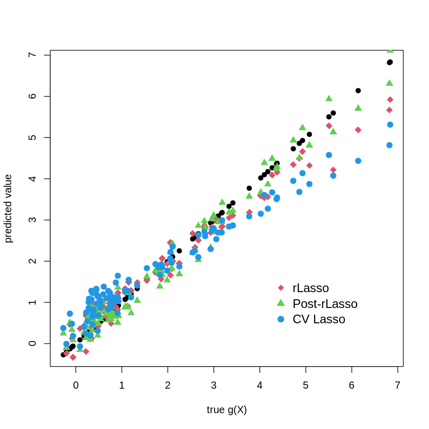
plot(gX, gX, pch=19, cex=1, ylab="predicted value", xlab="true g(X)")

points(gX, yhat.rlasso, col=2, pch=18, cex = 1.5 )
points(gX,  yhat.rlasso.post, col=3, pch=17,  cex = 1.2  )
points( gX, yhat.lasso.cv,col=4, pch=19,  cex = 1.2 )


legend("bottomright",
  legend = c("rLasso", "Post-rLasso", "CV Lasso"),
  col = c(2,3,4),
  pch = c(18,17, 19),
  bty = "n",
  pt.cex = 1.3,
  cex = 1.2,
  text.col = "black",
  horiz = F ,
  inset = c(0.1, 0.1))

7.2. Data Generating Process: Approximately Sparse + Small Dense Part#
set.seed(1)

n = 100;
p = 400;

Z= runif(n)-1/2;
W = matrix(runif(n*p)-1/2, n, p);


beta = rnorm(p)*.2    # dense beta
gX = exp(4*Z)+ W%*%beta;  # leading term nonlinear
X = cbind(Z, Z^2, Z^3, W );  # polynomials in Zs will be approximating exp(4*Z)


Y = gX + rnorm(n);    #generate Y


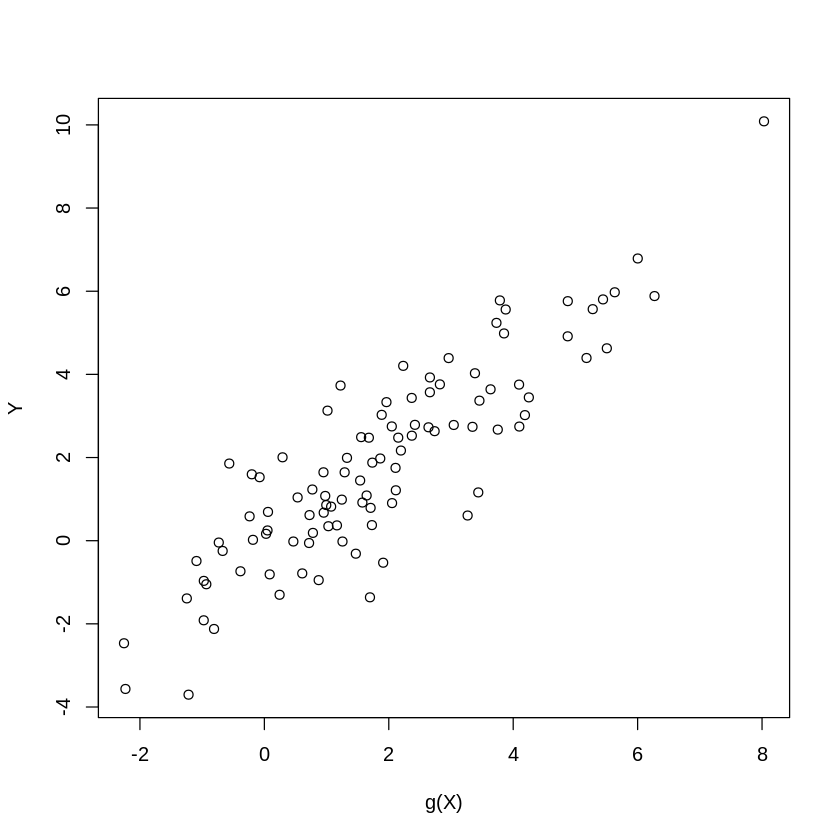
plot(gX,Y, xlab="g(X)", ylab="Y")    #plot V vs g(X)

print( c("theoretical R2:", var(gX)/var(Y)))
[1] "theoretical R2:" "0.696687990094227"
| 0.696688 |

# library(glmnet)
fit.lasso.cv   <- cv.glmnet(X, Y, family="gaussian", alpha=1)  # family gaussian means that we'll be using square loss
fit.ridge   <- cv.glmnet(X, Y, family="gaussian", alpha=0)     # family gaussian means that we'll be using square loss
fit.elnet   <- cv.glmnet(X, Y, family="gaussian", alpha=.5)    # family gaussian means that we'll be using square loss

yhat.lasso.cv    <- predict(fit.lasso.cv, newx = X)            # predictions
yhat.ridge   <- predict(fit.ridge, newx = X)
yhat.elnet   <- predict(fit.elnet, newx = X)

MSE.lasso.cv <- summary(lm((gX-yhat.lasso.cv)^2~1))$coef[1:2]  # report MSE and standard error for MSE for approximating g(X)
MSE.ridge <- summary(lm((gX-yhat.ridge)^2~1))$coef[1:2]        # report MSE and standard error for MSE for approximating g(X)
MSE.elnet <- summary(lm((gX-yhat.elnet)^2~1))$coef[1:2]        # report MSE and standard error for MSE for approximating g(X)
# library(hdm)
fit.rlasso  <- rlasso(Y~X,  post=FALSE)      # lasso with plug-in penalty level
fit.rlasso.post <- rlasso(Y~X,  post=TRUE)    # post-lasso with plug-in penalty level

yhat.rlasso   <- predict(fit.rlasso)            #predict g(X) for values of X
yhat.rlasso.post   <- predict(fit.rlasso.post)  #predict g(X) for values of X

MSE.lasso <- summary(lm((gX-yhat.rlasso)^2~1))$coef[1:2]       # report MSE and standard error for MSE for approximating g(X)
MSE.lasso.post <- summary(lm((gX-yhat.rlasso.post)^2~1))$coef[1:2]  # report MSE and standard error for MSE for approximating g(X)
# library(glmnet)

lava.predict<- function(X,Y, iter=5){

g1 = predict(rlasso(X, Y, post=F))  #lasso step fits "sparse part"
m1 =  predict(glmnet(X, as.vector(Y-g1), family="gaussian", alpha=0, lambda =20),newx=X ) #ridge step fits the "dense" part


i=1
while(i<= iter) {
  g1 = predict(rlasso(X, as.vector(Y-m1), post=F))   #lasso step fits "sparse part"
  m1 = predict(glmnet(X, as.vector(Y-g1), family="gaussian",  alpha=0, lambda =20),newx=X );  #ridge step fits the "dense" part
  i = i+1
}

return(g1+m1);
}


yhat.lava = lava.predict(X,Y)
MSE.lava <- summary(lm((gX-yhat.lava)^2~1))$coef[1:2]       # report MSE and standard error for MSE for approximating g(X)


MSE.lava
- 0.679714730890029
- 0.0737496772656864
# library(xtable)
table<- matrix(0, 6, 2)
table[1,1:2]   <- MSE.lasso.cv
table[2,1:2]   <- MSE.ridge
table[3,1:2]   <- MSE.elnet
table[4,1:2]   <- MSE.lasso
table[5,1:2]   <- MSE.lasso.post
table[6,1:2]   <- MSE.lava

colnames(table)<- c("MSA", "S.E. for MSA")
rownames(table)<- c("Cross-Validated Lasso", "Cross-Validated ridge","Cross-Validated elnet",
                    "Lasso","Post-Lasso","Lava")
# tab <- xtable(table, digits =3)

table
| MSA | S.E. for MSA | |
|---|---|---|
| Cross-Validated Lasso | 1.9318225 | 0.29130485 |
| Cross-Validated ridge | 3.4106685 | 0.49426500 |
| Cross-Validated elnet | 1.8251591 | 0.25189955 |
| Lasso | 0.9641151 | 0.11978038 |
| Post-Lasso | 1.5966018 | 0.20707956 |
| Lava | 0.6797147 | 0.07374968 |
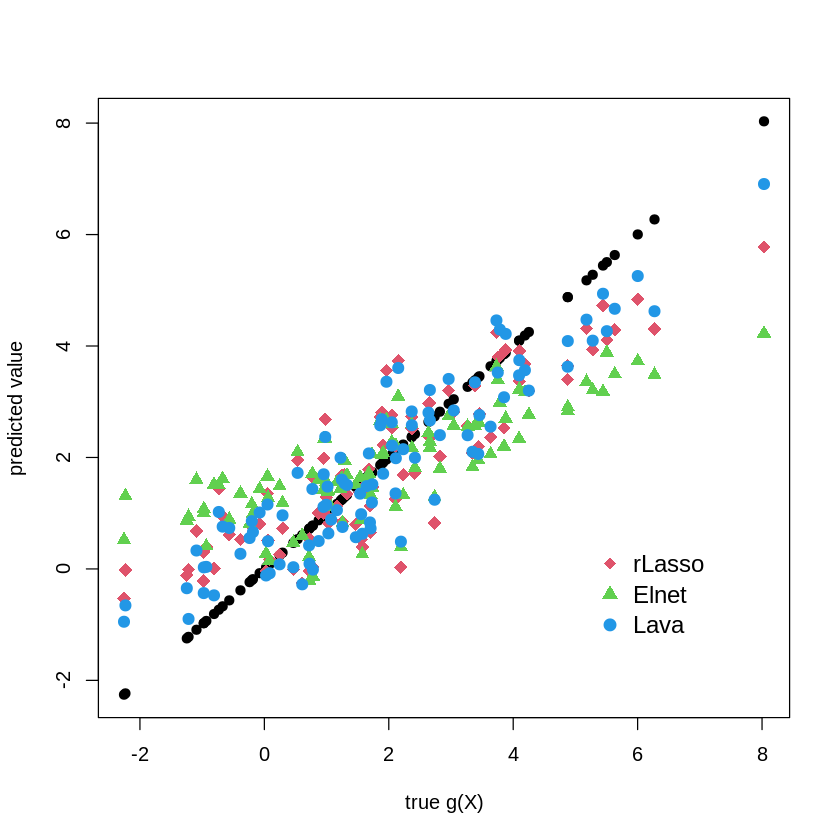
plot(gX, gX, pch=19, cex=1, ylab="predicted value", xlab="true g(X)")

points(gX, yhat.rlasso,   col=2, pch=18, cex = 1.5 )
points(gX, yhat.elnet,  col=3, pch=17,  cex = 1.2  )
points(gX, yhat.lava,  col=4, pch=19,  cex = 1.2 )


legend("bottomright",
  legend = c("rLasso", "Elnet", "Lava"),
  col = c(2,3,4),
  pch = c(18,17, 19),
  bty = "n",
  pt.cex = 1.3,
  cex = 1.2,
  text.col = "black",
  horiz = F ,
  inset = c(0.1, 0.1))


