23. Sensitivity Analysis with Sensmakr and Debiased ML#
23.1. Here we experiment with using package “sensemakr” in conjunction with debiased ML#
References:
Linear Models: Cinelli and Hazlett https://doi.org/10.1111/rssb.12348
Partially Linear and Nonlinear Models. Chernozhukov, Cinelli, Newey, Sharma, Syrgkanis https://arxiv.org/pdf/2112.13398.pdf
We will mimic the partialling out procedure with machine learning tools, and invoke Sensmakr to compute \(\phi^2\) and plot sensitivity results.
# loads package

install.packages("librarian")
librarian::shelf(
  sensemakr, hdm, lfe, randomForest, zoo
  , survival
)

# loads data
data("darfur")
Installing package into ‘/usr/local/lib/R/site-library’
(as ‘lib’ is unspecified)
Data is described here https://cran.r-project.org/web/packages/sensemakr/vignettes/sensemakr.html
The main outcome is attitude towards peace – the peacefactor. The key variable of interest is whether the responders were directly harmed (directlyharmed). We want to know if being directly harmed in the conflict causes people to support peace-enforcing measures. The measured confounders include female indicator, age, farmer, herder, voted in the past, and household size. There is also a village indicator, which we will treat as fixed effect and partial it out before conducting the analysis. The standard errors will be clustered at the village level.
23.2. Take out village fixed effects and run basic linear analysis#
#get rid of village fixed effects

attach(darfur)
# library(lfe)

peacefactorR<- lm(peacefactor~village)$res
directlyharmedR<-  lm(directlyharmed~village)$res
femaleR<-  lm(female~village)$res
ageR<-     lm(age~village)$res
farmerR<-  lm(farmer_dar~village)$res
herderR<-  lm(herder_dar~village)$res
pastvotedR<- lm(pastvoted~village)$res
hhsizeR<-   lm(hhsize_darfur~village)$res


# Preliminary linear model analysis

summary(felm(peacefactorR~ directlyharmedR+ femaleR +
                     ageR + farmerR+ herderR + pastvotedR + hhsizeR |0|0|village))

# here we are clustering standard errors at the village level


summary(felm(peacefactorR~ femaleR +
                     ageR + farmerR+ herderR + pastvotedR + hhsizeR |0|0|village))

# here we are clustering standard errors at the village level


summary(felm(directlyharmedR~ femaleR +
                     ageR + farmerR+ herderR + pastvotedR + hhsizeR |0|0|village))

# here we are clustering standard errors at the village level
Call:
   felm(formula = peacefactorR ~ directlyharmedR + femaleR + ageR +      farmerR + herderR + pastvotedR + hhsizeR | 0 | 0 | village)

Residuals:
     Min       1Q   Median       3Q      Max
-0.67487 -0.14712  0.00000  0.09857  0.90307

Coefficients:
                  Estimate Cluster s.e. t value Pr(>|t|)
(Intercept)     -7.428e-19    2.065e-17  -0.036  0.97131
directlyharmedR  9.732e-02    2.382e-02   4.085 4.68e-05 ***
femaleR         -2.321e-01    2.444e-02  -9.495  < 2e-16 ***
ageR            -2.072e-03    7.441e-04  -2.784  0.00545 **
farmerR         -4.044e-02    2.956e-02  -1.368  0.17156
herderR          1.428e-02    3.650e-02   0.391  0.69569
pastvotedR      -4.802e-02    2.688e-02  -1.787  0.07420 .
hhsizeR          1.230e-03    2.166e-03   0.568  0.57034
---
Signif. codes:  0 ‘***’ 0.001 ‘**’ 0.01 ‘*’ 0.05 ‘.’ 0.1 ‘ ’ 1

Residual standard error: 0.2437 on 1268 degrees of freedom
Multiple R-squared(full model): 0.1542   Adjusted R-squared: 0.1496
Multiple R-squared(proj model): 0.1542   Adjusted R-squared: 0.1496
F-statistic(full model, *iid*):33.03 on 7 and 1268 DF, p-value: < 2.2e-16
F-statistic(proj model): 25.44 on 7 and 485 DF, p-value: < 2.2e-16
Call:
   felm(formula = peacefactorR ~ femaleR + ageR + farmerR + herderR +      pastvotedR + hhsizeR | 0 | 0 | village)

Residuals:
     Min       1Q   Median       3Q      Max
-0.63765 -0.15168  0.00000  0.09859  0.90298

Coefficients:
              Estimate Cluster s.e. t value Pr(>|t|)
(Intercept) -1.375e-18    1.991e-17  -0.069  0.94496
femaleR     -2.415e-01    2.536e-02  -9.522  < 2e-16 ***
ageR        -2.187e-03    7.453e-04  -2.934  0.00341 **
farmerR     -4.071e-02    2.923e-02  -1.393  0.16390
herderR      2.623e-02    3.968e-02   0.661  0.50871
pastvotedR  -4.414e-02    2.784e-02  -1.585  0.11313
hhsizeR      1.336e-03    2.127e-03   0.628  0.52991
---
Signif. codes:  0 ‘***’ 0.001 ‘**’ 0.01 ‘*’ 0.05 ‘.’ 0.1 ‘ ’ 1

Residual standard error: 0.2463 on 1269 degrees of freedom
Multiple R-squared(full model): 0.1353   Adjusted R-squared: 0.1312
Multiple R-squared(proj model): 0.1353   Adjusted R-squared: 0.1312
F-statistic(full model, *iid*): 33.1 on 6 and 1269 DF, p-value: < 2.2e-16
F-statistic(proj model): 23.07 on 6 and 485 DF, p-value: < 2.2e-16
Call:
   felm(formula = directlyharmedR ~ femaleR + ageR + farmerR + herderR +      pastvotedR + hhsizeR | 0 | 0 | village)

Residuals:
    Min      1Q  Median      3Q     Max
-0.8285 -0.3129  0.0000  0.2630  0.9076

Coefficients:
              Estimate Cluster s.e. t value Pr(>|t|)
(Intercept) -8.331e-18    2.684e-17  -0.310   0.7563
femaleR     -9.714e-02    5.129e-02  -1.894   0.0585 .
ageR        -1.182e-03    1.151e-03  -1.028   0.3044
farmerR     -2.789e-03    4.280e-02  -0.065   0.9481
herderR      1.228e-01    5.064e-02   2.425   0.0155 *
pastvotedR   3.991e-02    3.366e-02   1.186   0.2360
hhsizeR      1.093e-03    3.286e-03   0.333   0.7394
---
Signif. codes:  0 ‘***’ 0.001 ‘**’ 0.01 ‘*’ 0.05 ‘.’ 0.1 ‘ ’ 1

Residual standard error: 0.3744 on 1269 degrees of freedom
Multiple R-squared(full model): 0.0179   Adjusted R-squared: 0.01326
Multiple R-squared(proj model): 0.0179   Adjusted R-squared: 0.01326
F-statistic(full model, *iid*):3.856 on 6 and 1269 DF, p-value: 0.0008089
F-statistic(proj model): 3.828 on 6 and 485 DF, p-value: 0.0009698
23.3. We first use Lasso for Partilling Out Controls#
# library(hdm)


resY =  rlasso(peacefactorR ~  (femaleR +
                     ageR + farmerR+ herderR + pastvotedR + hhsizeR)^3, post=F)$res

resD =  rlasso(directlyharmedR ~  (femaleR +
                     ageR + farmerR + herderR + pastvotedR + hhsizeR)^3 , post=F)$res


print(c("Controls explain the following fraction of variance of Outcome", 1-var(resY)/var(peacefactorR)))


print(c("Controls explain the following fraction of variance of Treatment", 1-var(resD)/var(directlyharmedR)))


# library(lfe)


dml.darfur.model= felm(resY ~ resD|0|0|village)   # cluster SEs by village

summary(dml.darfur.model,robust=T)  #culster SE by village

dml.darfur.model= lm(resY ~ resD)  #lineaer model to use as input in sensemakr
[1] "Controls explain the following fraction of variance of Outcome"
[2] "0.125108054898996"
[1] "Controls explain the following fraction of variance of Treatment"
[2] "0.0119842379295265"
Call:
   felm(formula = resY ~ resD | 0 | 0 | village)

Residuals:
     Min       1Q   Median       3Q      Max
-0.63410 -0.15299  0.00069  0.09305  0.89593

Coefficients:
             Estimate Cluster s.e. t value Pr(>|t|)
(Intercept) 5.763e-18    1.594e-04   0.000        1
resD        1.003e-01    2.443e-02   4.108 4.25e-05 ***
---
Signif. codes:  0 ‘***’ 0.001 ‘**’ 0.01 ‘*’ 0.05 ‘.’ 0.1 ‘ ’ 1

Residual standard error: 0.2444 on 1274 degrees of freedom
Multiple R-squared(full model): 0.02312   Adjusted R-squared: 0.02235
Multiple R-squared(proj model): 0.02312   Adjusted R-squared: 0.02235
F-statistic(full model, *iid*):30.15 on 1 and 1274 DF, p-value: 4.82e-08
F-statistic(proj model): 16.87 on 1 and 485 DF, p-value: 4.693e-05
23.4. Manual Bias Analysis#
# Main estimate

beta = dml.darfur.model$coef[2]

# Hypothetical values of partial R2s

R2.YC = .16; R2.DC = .01

# Elements of the formal

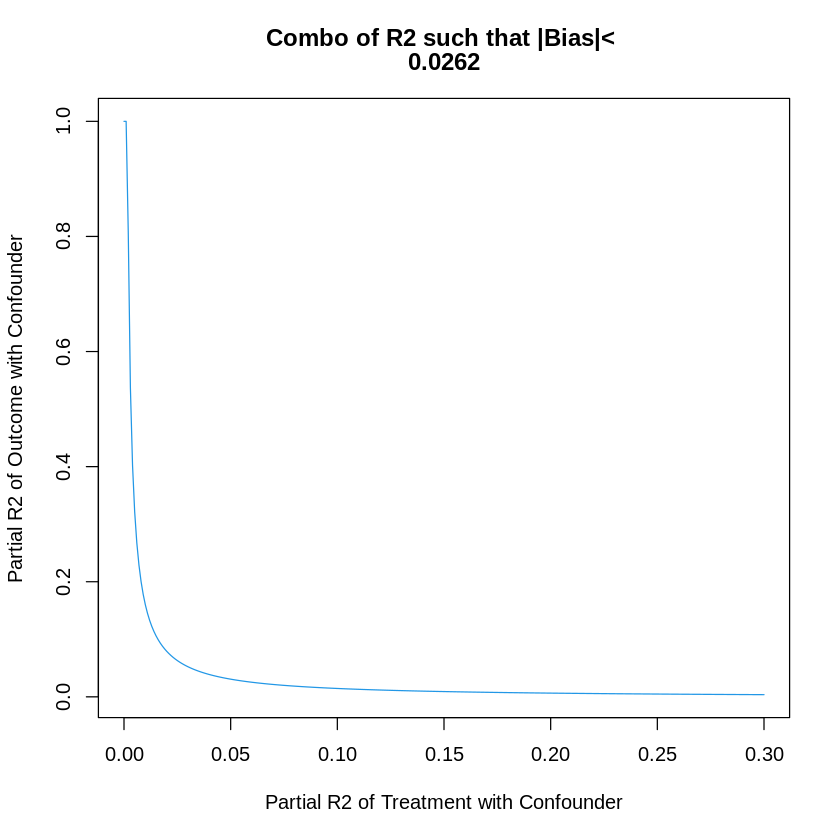
kappa<-  (R2.YC * R2.DC)/(1- R2.DC)

varianceRatio<- mean(dml.darfur.model$res^2)/mean(resD^2)

# Compute square bias

BiasSq <-  kappa*varianceRatio

# Compute absolute value of the bias

print(sqrt(BiasSq))


# plotting

gridR2.DC<- seq(0,.3, by=.001)

gridR2.YC<- kappa*(1 - gridR2.DC)/gridR2.DC

gridR2.YC<- ifelse(gridR2.YC> 1, 1, gridR2.YC);


plot(gridR2.DC, gridR2.YC, type="l", col=4, xlab="Partial R2 of Treatment with Confounder",
     ylab="Partial R2 of Outcome with Confounder",
    main= c("Combo of R2 such that |Bias|< ", round(sqrt(BiasSq), digits=4))
)
[1] 0.02622016

23.5. Bias Analysis with Sensemakr#
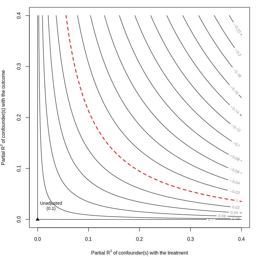
dml.darfur.sensitivity <- sensemakr(model = dml.darfur.model,
                                treatment = "resD")
summary(dml.darfur.sensitivity)

plot(dml.darfur.sensitivity, nlevels = 15)
Sensitivity Analysis to Unobserved Confounding

Model Formula: resY ~ resD

Null hypothesis: q = 1 and reduce = TRUE
-- This means we are considering biases that reduce the absolute value of the current estimate.
-- The null hypothesis deemed problematic is H0:tau = 0

Unadjusted Estimates of 'resD':
  Coef. estimate: 0.1003
  Standard Error: 0.0183
  t-value (H0:tau = 0): 5.491

Sensitivity Statistics:
  Partial R2 of treatment with outcome: 0.0231
  Robustness Value, q = 1: 0.1425
  Robustness Value, q = 1, alpha = 0.05: 0.0941

Verbal interpretation of sensitivity statistics:

-- Partial R2 of the treatment with the outcome: an extreme confounder (orthogonal to the covariates) that explains 100% of the residual variance of the outcome, would need to explain at least 2.31% of the residual variance of the treatment to fully account for the observed estimated effect.

-- Robustness Value, q = 1: unobserved confounders (orthogonal to the covariates) that explain more than 14.25% of the residual variance of both the treatment and the outcome are strong enough to bring the point estimate to 0 (a bias of 100% of the original estimate). Conversely, unobserved confounders that do not explain more than 14.25% of the residual variance of both the treatment and the outcome are not strong enough to bring the point estimate to 0.

-- Robustness Value, q = 1, alpha = 0.05: unobserved confounders (orthogonal to the covariates) that explain more than 9.41% of the residual variance of both the treatment and the outcome are strong enough to bring the estimate to a range where it is no longer 'statistically different' from 0 (a bias of 100% of the original estimate), at the significance level of alpha = 0.05. Conversely, unobserved confounders that do not explain more than 9.41% of the residual variance of both the treatment and the outcome are not strong enough to bring the estimate to a range where it is no longer 'statistically different' from 0, at the significance level of alpha = 0.05.

23.6. Next We use Random Forest as ML tool for Partialling Out#
The following code does DML with clsutered standard errors by ClusterID
DML2.for.PLM <- function(x, d, y, dreg, yreg, nfold=2, clusterID) {
  nobs <- nrow(x) #number of observations
  foldid <- rep.int(1:nfold,times = ceiling(nobs/nfold))[sample.int(nobs)] #define folds indices
  I <- split(1:nobs, foldid)  #split observation indices into folds
  ytil <- dtil <- rep(NA, nobs)
  cat("fold: ")
  for(b in 1:length(I)){
    dfit <- dreg(x[-I[[b]],], d[-I[[b]]]) #take a fold out
    yfit <- yreg(x[-I[[b]],], y[-I[[b]]]) # take a foldt out
    dhat <- predict(dfit, x[I[[b]],], type="response") #predict the left-out fold
    yhat <- predict(yfit, x[I[[b]],], type="response") #predict the left-out fold
    dtil[I[[b]]] <- (d[I[[b]]] - dhat) #record residual for the left-out fold
    ytil[I[[b]]] <- (y[I[[b]]] - yhat) #record residial for the left-out fold
    cat(b," ")
        }
  rfit <- felm(ytil ~ dtil |0|0|clusterID)    #get clustered standard errors using felm
  rfitSummary<- summary(rfit)
  coef.est <-  rfitSummary$coef[2] #extract coefficient
  se <- rfitSummary$coef[2,2]  #record robust standard error
  cat(sprintf("\ncoef (se) = %g (%g)\n", coef.est , se))  #printing output
  return( list(coef.est =coef.est , se=se, dtil=dtil, ytil=ytil) ) #save output and residuals
}
x= model.matrix(~  femaleR + ageR + farmerR + herderR + pastvotedR + hhsizeR)

dim(x)

d= directlyharmedR

y = peacefactorR;

#DML with Random Forest:
dreg <- function(x,d){ randomForest(x, d) } #ML method=Forest
yreg <- function(x,y){ randomForest(x, y) } #ML method=Forest
set.seed(1)
DML2.RF = DML2.for.PLM(x, d, y, dreg, yreg, nfold=10, clusterID=village)


resY =  DML2.RF$ytil

resD =  DML2.RF$dtil


print(c("Controls explain the following fraction of variance of Outcome", max(1-var(resY)/var(peacefactorR),0)))


print(c("Controls explain the following fraction of variance of Treatment", max(1-var(resD)/var(directlyharmedR),0)))


dml.darfur.model= lm(resY~resD)


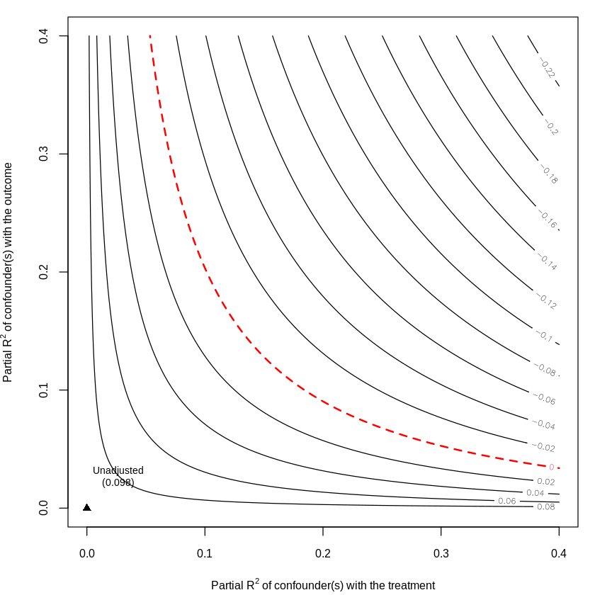
dml.darfur.sensitivity <- sensemakr(model = dml.darfur.model,
                                treatment = "resD")
summary(dml.darfur.sensitivity)

plot(dml.darfur.sensitivity,nlevels = 15)
- 1276
- 7
fold: 1  2  3  4  5  6  7  8  9  10
coef (se) = 0.097853 (0.0248297)
[1] "Controls explain the following fraction of variance of Outcome"
[2] "0.0451160320722748"
[1] "Controls explain the following fraction of variance of Treatment"
[2] "0"
Sensitivity Analysis to Unobserved Confounding

Model Formula: resY ~ resD

Null hypothesis: q = 1 and reduce = TRUE
-- This means we are considering biases that reduce the absolute value of the current estimate.
-- The null hypothesis deemed problematic is H0:tau = 0

Unadjusted Estimates of 'resD':
  Coef. estimate: 0.0979
  Standard Error: 0.0182
  t-value (H0:tau = 0): 5.3655

Sensitivity Statistics:
  Partial R2 of treatment with outcome: 0.0221
  Robustness Value, q = 1: 0.1394
  Robustness Value, q = 1, alpha = 0.05: 0.0909

Verbal interpretation of sensitivity statistics:

-- Partial R2 of the treatment with the outcome: an extreme confounder (orthogonal to the covariates) that explains 100% of the residual variance of the outcome, would need to explain at least 2.21% of the residual variance of the treatment to fully account for the observed estimated effect.

-- Robustness Value, q = 1: unobserved confounders (orthogonal to the covariates) that explain more than 13.94% of the residual variance of both the treatment and the outcome are strong enough to bring the point estimate to 0 (a bias of 100% of the original estimate). Conversely, unobserved confounders that do not explain more than 13.94% of the residual variance of both the treatment and the outcome are not strong enough to bring the point estimate to 0.

-- Robustness Value, q = 1, alpha = 0.05: unobserved confounders (orthogonal to the covariates) that explain more than 9.09% of the residual variance of both the treatment and the outcome are strong enough to bring the estimate to a range where it is no longer 'statistically different' from 0 (a bias of 100% of the original estimate), at the significance level of alpha = 0.05. Conversely, unobserved confounders that do not explain more than 9.09% of the residual variance of both the treatment and the outcome are not strong enough to bring the estimate to a range where it is no longer 'statistically different' from 0, at the significance level of alpha = 0.05.


